

Geographic Information Systems (GIS) have fundamentally changed how organizations analyze spatial patterns, manage land, model environmental impacts, and design urban infrastructure. At the center of this spatial revolution is Esri, whose industry-standard software suite provides unparalleled analytical depth. Whether you are transitioning to ArcGIS Pro or stepping into spatial analytics for the first time, learning how to leverage essential ArcGIS tools is critical to unlocking actionable insights from geographical data.
The software offers hundreds of specialized utilities, but mastering a core set of foundational functions can solve nearly eighty percent of real-world spatial challenges. This guide offers a comprehensive, expert-level breakdown of the essential ArcGIS tools every practitioner should master, highlighting their core mechanics, practical application scenarios, and key technical considerations. By integrating these top geoprocessing tools for beginner GIS analysts and seasoned spatial data scientists alike, you will streamline your workflows, ensure accurate geometric results, and harness the true potential of GIS spatial analysis software.
Table of Contents
Vector Analysis Tools: The Foundation of Spatial Proximity and Overlays
Vector data—comprising points, lines, and polygons—represents discrete geographic features across the globe. Analyzing vector relationships requires precise operations that measure proximity, define intersecting regions, and extract specific spatial subsets. Here are the core ArcGIS Pro geoprocessing tools required for vector analysis.
The Buffer Tool: Proximity and Environmental Impact Modeling
The Buffer tool is arguably one of the most fundamental vector analysis utilities in ArcGIS. At its core, the Buffer tool creates polygon boundaries at a specified distance around input point, line, or polygon features. This tool is essential for establishing zones of influence, environmental setbacks, or accessibility perimeters.
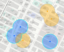
When executing a buffer operation, analysts specify a fixed distance or choose an attribute table field that contains varying buffer distances per feature. Advanced buffer parameters allow for geodesic buffering, which accounts for the Earth’s curvature over large geographical expanses, avoiding distortion caused by planar coordinate projections. Key parameters include the side type (full, left, right) for line features and the end type (round or flat). Analysts can also elect to dissolve overlapping buffer polygons into a single contiguous feature, which prevents double-counting areas during subsequent spatial joins or surface calculations. Typical use cases include mapping noise protection zones around airports, establishing stream protection corridors for watershed management, or defining walking catchments surrounding transit hubs.
Spatial Join: Merging Data Attributes Based on Geographic Location
While traditional database joins rely on matching common alphanumeric keys across tables, the Spatial Join tool connects attributes from one layer to another based on spatial relationships. It answers the fundamental question: What is located where, and what features overlap or contain another feature?
Spatial Join provides several match options, including Intersect, Within a Distance, Contains, Completely Contains, Within, and Completely Within. When performing a spatial join, you can specify one-to-one or one-to-many relationships. For one-to-one joins, merge rules dictate how target attributes summarize incoming data—allowing you to calculate mean, sum, minimum, or maximum values across intersecting entities. For example, a spatial analyst can join demographic census block data directly to municipal parcel polygons, or summarize the total number of crime events occurring inside distinct police precinct boundaries. Understanding spatial join behavior is crucial for aggregating point data into administrative polygons without relying on manually entered spatial IDs.
Intersect and Union: Precise Geometric Overlays
Geometric overlay tools allow GIS analysts to combine distinct vector layers to determine geometric intersections and logical unions.
The Intersect tool computes the geometric intersection of two or more input feature layers. The output contains only those portions of features that overlap across all inputs, inheriting the combined attribute tables of every participating layer. This tool is crucial for multi-criteria suitability evaluations—for example, finding areas that are simultaneously classified as prime agricultural soil, zoned for commercial development, and situated outside designated floodplains.
Conversely, the Union tool calculates a geometric stack of polygon layers, preserving all features and attributes from all input datasets. Portions of features that do not overlap are still included in the final output dataset, populated with null values for fields originating from non-overlapping layers. The Union tool is widely used in land-use planning, environmental boundary consolidation, and risk assessment mapping, making it one of the best ArcGIS tools for spatial analysis when evaluating complete coverage scenarios.
Clip and Select By Location: Data Extraction Techniques
Managing large spatial datasets requires efficient tools for isolating areas of interest. The Clip tool acts like a spatial cookie cutter, trimming a vector layer using the boundary of another polygon dataset. Unlike the Intersect tool, the Clip tool preserves only the attributes of the input layer, ignoring attributes from the clipping boundary layer. This makes Clip ideal for cropping regional or national road networks, hydrography, or parcel datasets down to specific municipal boundaries.
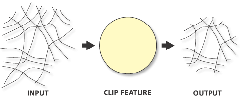
In contrast, the Select By Location tool selects features within a target layer based on their spatial relationship to a selecting layer (for instance, selecting all building footprints that fall within a 100-meter buffer of a river). Unlike Clip, Select By Location does not create a new output feature class on disk; instead, it generates an active selection set in the current map view, allowing for rapid interactive filtering, attribute calculation, or export.
Advanced Surface and Raster Analysis Tools
Raster data represents continuous spatial phenomena across grid cells, such as elevation, rainfall, temperature, and satellite imagery spectral response. Esri mapping capabilities shine brightest when executing grid-based calculations using Spatial Analyst tools.
Spatial Analyst Extension and Grid Operations
The Spatial Analyst module expands ArcGIS Pro into a powerful environment for grid-based continuous surface modeling. Raster analysis relies on cell dimensions, coordinate alignment, and spatial resolution. When running Spatial Analyst tools, establishing uniform Environment Settings—such as setting the Processing Extent, Snap Raster, and Cell Size—is imperative to maintain grid alignment and prevent spatial resampling artifacts across calculations.
Raster Calculator: Custom Map Algebra Formulas
The Raster Calculator is an indispensable tool for mathematical and logical map algebra operations. Utilizing a Python-based syntax interface, the Raster Calculator permits complex expressions involving multiple raster layers, scalar constants, trigonometric functions, and conditional evaluation logic.
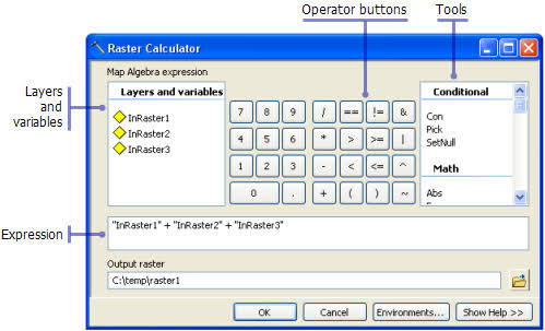
Analysts use the Raster Calculator to perform Normalized Difference Vegetation Index (NDVI) calculations from multi-spectral remote sensing imagery, execute Boolean overlay models for site suitability analysis, and convert unit measurement scales across continuous datasets. For instance, evaluating habitat suitability often requires combining weighted raster criteria (e.g., elevation, slope, canopy cover, distance to roads) into a single composite index score using explicit mathematical formulas.
Topographic Analysis: Slope, Aspect, and Hillshade
Digital Elevation Models (DEMs) are foundational raster datasets that model ground elevation values across continuous terrain. ArcGIS provides specialized terrain analysis tools to extract crucial geomorphological properties from DEMs:
- Slope: Calculates the rate of maximum elevation change across adjacent cells, expressing output in degrees or percentage rise. Slope mapping is vital for landslide risk modeling, agricultural runoff analysis, and road grade planning.
- Aspect: Identifies the compass direction that the maximum rate of change in value from each cell to its neighbors faces. Aspect values indicate terrain orientation (North, South, East, West), which directly impacts solar radiation exposure, snowmelt rates, and vegetation growth distribution.
- Hillshade: Computes surface illumination by simulating a light source position (azimuth and altitude) across the DEM terrain. The resulting grayscale raster produces a visually compelling representation of terrain relief, dramatically improving map visualization quality and shaded relief mapping.
Interpolation Tools: IDW, Kriging, and Spline
Real-world data collection often relies on discrete point measurements, such as weather station readings, soil sample contents, or air quality monitoring sensors. Interpolation tools convert discrete point data into continuous surface rasters by estimating missing values between sample points.
- Inverse Distance Weighted (IDW): Assumes that features closer to one another are more alike than those further apart. IDW calculates cell values using a weighted average of surrounding sample points, where the weight decreases as distance to the target cell increases.
- Kriging: An advanced geostatistical interpolation method that models both spatial distance and directional spatial auto-correlation. Kriging provides statistical measure of prediction certainty or uncertainty across the estimated surface, making it superior for geological exploration and meteorology.
- Spline: Fits a mathematical surface through sample points while minimizing total surface curvature, yielding smooth continuous rasters suitable for gentle elevation trends or temperature surfaces.
Data Management, Attribute Handling, and Layer Cleanup
Spatial analytics depends heavily on clean, normalized spatial and non-spatial tabular data. Effective database management ensures that spatial operations run smoothly and return accurate spatial metrics.
Table Joins and Relates: Connecting Enterprise Information
Geodatabase tables frequently isolate tabular non-spatial records from geographic feature classes. The Add Join tool establishes a relational connection between a spatial layer’s attribute table and an external stand-alone table based on a shared common key field.
When joining tables, field data types must match precisely (e.g., Integer to Integer, or String to String). In contrast to a permanent merge, an attribute join is dynamic; the original source tables remain unchanged while the map interface displays a unified table view. When one-to-many or many-to-many spatial relationships exist, using a Relate or Relate Class is preferred over a join, allowing users to navigate linked records interactively without duplicating geometric features.
Dissolve: Aggregating Vector Features
Over the course of GIS analysis, boundary detail can become redundant or overly complex. The Dissolve tool aggregates features that share the same attribute value across specified dissolve fields.
For instance, if a dataset contains thousands of individual county polygons with state name attributes, running the Dissolve tool grouped by the state field generates fifty statewide boundary polygons. During the dissolve operation, analysts can summarize numeric attributes of merged features—computing total population sums, average income statistics, or maximum elevation values across aggregated boundaries.
Field Calculator: Advanced Data Formatting and Mathematical Operations
The Field Calculator is an essential utility for creating, updating, and formatting attributes within vector layer attribute tables. Supported by Python and Arcade expression engines, the Field Calculator allows analysts to execute complex string processing, mathematical operations, date calculations, and logical conditions across thousands of rows instantly.
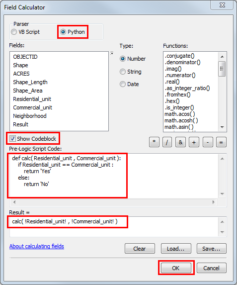
Common applications include string concatenation (combining separate street directional, name, and type fields into a single full address field), geometry measurement updates (calculating exact geodesic area or perimeter length in custom units), and conditional value reclassification using Python if-else logic. Mastering geometry calculations via the Field Calculator ensures that spatial metrics remain accurate after geometric editing or projection changes.
Automation and Workflow Optimization
Executing geoprocessing tools manually through user interfaces can become tedious and prone to human error when repeating workflows across multiple regions or time periods. ArcGIS Pro offers built-in visual and programmatic automation environments to streamline complex spatial analysis.
ModelBuilder: Creating Visual Geoprocessing Pipelines
ModelBuilder is a visual programming environment integrated directly into ArcGIS Pro. It allows users to build reusable workflows by linking data inputs, geoprocessing tools, and output datasets together on an interactive visual canvas.
In ModelBuilder, tools are represented as process blocks connected by directional arrows that define data flow. Key advantages of using ModelBuilder include:
- Workflow Standardization: Models document complex multi-step analytical processes visually, ensuring that methodologies can be reviewed, shared, and audited across teams.
- Iteration and Batch Processing: ModelBuilder features built-in iterators (e.g., Iterate Feature Classes, Iterate Workspaces) that allow analysts to repeat sequences automatically across hundreds of shapefiles or geodatabase layers without manual intervention.
- Integration with Model Parameters: By exposing input parameters, models can be saved as custom geoprocessing tools that colleagues can run using standard user interface dialogs.
ArcPy and Python Scripting: Advanced GIS Automation
For maximum control, scalability, and customization, Esri provides ArcPy—a dedicated Python site package. ArcPy enables users to call every ArcGIS geoprocessing tool programmatically, automate map document rendering, perform advanced cursor operations on attribute tables, and integrate third-party data science libraries like Pandas, NumPy, and SciPy.
Learning how to use essential tools in ArcGIS Pro through Python scripts allows GIS professionals to automate nightly database maintenance, conduct large-scale batch spatial analysis on cloud servers, and publish automated web mapping services. Python scripting transforms GIS analysts from software operators into efficient spatial data engineers capable of building end-to-end automated geospatial data pipelines.
Best Practices for Mastering ArcGIS Tools
To maximize performance, maintain precision, and avoid common technical errors while using essential ArcGIS tools, follow these core professional guidelines:
- Maintain Projection Consistency: Always verify that your input data layers share a unified projected coordinate system suitable for your local study region before executing geometric operations like Buffer, Intersect, or Area Calculations. Operating across mismatched or geographic coordinate systems can lead to inaccurate distance calculations and severe visual distortion.
- Set Environment Parameters Thoughtfully: Always configure Geoprocessing Environment Settings before running analytical pipelines. Explicitly defining your Output Coordinate System, Processing Extent, Snap Raster, and Cell Size guarantees consistent alignment across all generated spatial outputs.
- Keep Geodatabase Architecture Clean: Avoid storing working datasets in transient temporary locations without clear naming conventions. Utilize file geodatabases (.gdb) or enterprise geodatabases over outdated legacy shapefiles, as geodatabases support longer field names, domain rules, topology checks, and larger file sizes.
- Leverage Spatial Indexes: For massive spatial datasets containing millions of point or polygon features, ensure that spatial indexes are built and updated. Spatial indexing dramatically accelerates spatial query speeds, Select By Location operations, and spatial join performance.
Conclusion
Mastering the essential ArcGIS tools detailed in this guide provides the core foundation for professional spatial analysis, map visualization, and geographic decision-making. From basic vector operations like buffering and spatial joins to advanced grid algebra via the Raster Calculator and automated workflow construction using ModelBuilder, these geoprocessing capabilities turn raw spatial data into powerful insights.
As geographic data continues to expand in volume and complexity, the ability to select the right GIS tool for the task—and chain those tools together effectively—remains the hallmark of a skilled GIS professional. By committing these core tools and best practices to memory, you will dramatically increase your analytical efficiency, produce reproducible scientific results, and unlock the full capabilities of the ArcGIS ecosystem.