Mastering ArcGIS Buffer Tool – A Comprehensive Guide to Proximity Analysis in GIS

In Geographic Information Systems (GIS), space is the fundamental fabric through which real-world spatial phenomena are organized, evaluated, and understood. Among the vast ecosystem of geoprocessing capabilities available to analysts, proximity analysis stands as one of the most critical foundational workflows. At the heart of proximity analysis lies a remarkably versatile tool: the ArcGIS buffer tool. Whether you are an urban planner evaluating access to public transit, an environmental scientist establishing protection zones around pristine waterways, a retail site analyst calculating customer catchment areas, or a public safety coordinator mapping emergency evacuation perimeters, buffering is an indispensable routine.

Despite its conceptual simplicity—creating a polygon at a specified distance around an input feature—the ArcGIS buffer tool encompasses a sophisticated array of options, mathematical models, and spatial parameters. A surface-level understanding of this tool can lead to significant spatial inaccuracies, distorted analytical conclusions, and improper map representations. For example, choosing between Euclidean distance and geodesic distance, selecting appropriate end cap styles, or determining whether to dissolve overlapping boundaries can fundamentally alter the output of your spatial analysis.

This comprehensive guide provides an in-depth exploration of the ArcGIS buffer tool within both ArcGIS Pro and ArcMap environments. We will demystify core buffering concepts, differentiate between geometric methods, walk through step-by-step execution workflows, examine advanced parameters, explore the multi ring buffer arcgis capability, and outline real-world applications and troubleshooting techniques. By the end of this tutorial, you will possess the expert knowledge necessary to execute precise, mathematically sound buffer analysis in arcgis for any spatial challenge.

What is the ArcGIS Buffer Tool?

At its core, the ArcGIS buffer tool is a fundamental geoprocessing tool designed to create vector polygon layers around input vector features—points, lines, or polygons—at a user-specified offset distance. The primary objective of buffer analysis in GIS is to delineate spatial boundaries based on proximity, establishing dynamic zones of influence or interest around geographic entities.

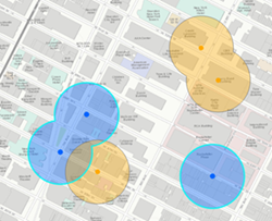
When you execute a buffer operation, the software calculates geometric offsets from the boundaries or coordinates of the input feature layer. For point features, a fixed-distance buffer generates a circle centered on the point coordinate. For line features, the tool creates a parallel corridor offset by the specified buffer distance along both sides of the line, rounded or flattened at the extremities depending on settings. For polygon features, the buffer extends outward (or inward) from the existing polygon boundary, expanding the spatial envelope by the designated measurement.

The ArcGIS buffer tool supports two foundational modes of distance designation: fixed distance buffering and variable distance buffering (attribute-driven buffering).

1. Fixed Distance Buffers: The user inputs a uniform static measurement (such as 500 meters, 1 mile, or 10 kilometers) that applies equally across every individual feature within the input dataset.
2. Variable Distance Buffers: The buffer distance is derived dynamically from a numeric field in the attribute table of the input feature layer. For instance, if you possess a dataset of fire stations with an attribute field indicating each station’s maximum response distance based on staffing levels, the buffer tool can generate distinct, customized buffer radii for each station in a single operation.

Understanding how geographic features interact within these offset zones allows analysts to execute effective gis proximity analysis to answer complex questions regarding spatial influence, accessibility, potential environmental impact, and spatial compliance.

Key Concepts: Geodesic vs. Euclidean Buffering

One of the most critical technical considerations when running the arcgis pro buffer tool is choosing between Planar (Euclidean) and Geodesic buffering methods. Selecting the wrong distance method can introduce profound spatial distortion, particularly when working with regional, national, or global datasets.

Euclidean Buffering (Planar Distance)

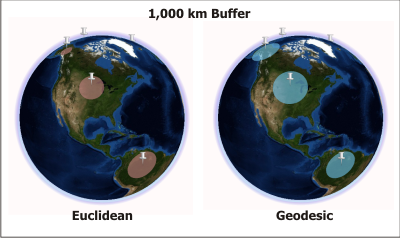
Euclidean buffering operates on a flat, two-dimensional Cartesian coordinate system. It assumes that the Earth’s surface is flat, measuring distances directly as a straight line between two points on a 2D plane. Euclidean buffering is computationally fast and highly accurate when performed over small, localized spatial areas using an appropriate projected coordinate system (PCS) designed for that region, such as a local State Plane Coordinate System or a narrow Universal Transverse Mercator (UTM) zone.

However, when Euclidean buffering is applied over large geographical regions, across UTM zone boundaries, or on layers using a geographic coordinate system (GCS) like WGS 1984, severe spatial distortion occurs. Because flat projections inevitably distort area, distance, shape, or direction as spatial extent increases, Euclidean buffers created over vast areas will not represent accurate real-world distances on the curved surface of the Earth.

Geodesic Buffering (Ellipsoidal Distance)

Geodesic buffering accounts for the three-dimensional, ellipsoidal shape of the Earth. Instead of treating map space as a flat sheet of paper, geodesic algorithms calculate distances directly along the surface of the Earth’s ellipsoid (the 3D shape defined by spatial reference standards like WGS 1984 or NAD 1983).

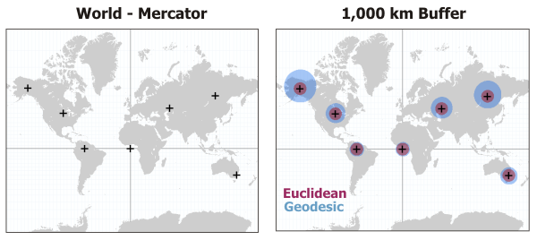
When you run a geodesic buffer, the result correctly accounts for the curvature of the Earth. If you map a 500-mile geodesic buffer around a point near the Equator and another around a point near the North Pole on a Mercator map projection, the polar buffer will appear visually larger and distorted on the 2D display. However, in true Earth surface measurements, both buffers enclose the exact same surface area.

Understanding the difference between geodesic and euclidean buffer arcgis settings is paramount for maintaining scientific accuracy:

• Use Planar/Euclidean Buffering: When working within localized map projections (such as city or county-level datasets) where planar measurements retain minimal distortion.
• Use Geodesic Buffering: Whenever your data covers large geographic extents (such as multi-state, continental, or global scales), or when working directly with unprojected spatial data in geographic coordinate systems.

Step-by-Step Guide: How to Create a Buffer in ArcGIS Pro

Executing a buffer operation in ArcGIS Pro is a fundamental skill every GIS analyst must master. Below is a detailed, step-by-step workflow describing how to create fixed distance buffer in arcgis pro using standard vector input layers.

Step 1: Access the Geoprocessing Pane

Launch ArcGIS Pro and open your project containing the relevant feature layers. Navigate to the top ribbon menu and click on the Analysis tab. From the Analysis tab, click on the Tools icon to launch the Geoprocessing pane on the right side of your workspace.

Step 2: Locate the Buffer Tool

In the Geoprocessing pane search bar, type “Buffer” and press Enter. Alternatively, you can locate the tool directly by navigating to Analysis Tools > Proximity > Buffer. Click on the Buffer tool to open its parameter configurations.

Step 3: Define Input Features and Output Feature Class

In the Input Features parameter drop-down menu, select the feature layer (point, line, or polygon) that you wish to buffer. Next, specify the path and filename for the Output Feature Class in your target geodatabase or folder directory. Ensure your naming convention clearly reflects the layer and distance (for example, Streams_Buffer_100m).

Step 4: Specify Distance Parameters

Under the Distance section, you can choose between a static distance measurement or an attribute field:

• Distance [value or field]: To execute a fixed distance buffer, select the radio button for Distance and enter a numeric value (such as 100). Next, select the linear unit of measure from the drop-down menu (such as Meters, Feet, Kilometers, or Miles).
• Field: If you want to perform variable distance buffering based on layer attributes, select Field and choose the numeric column that contains the specific offset distances for each feature.

Step 5: Select Side Type and End Cap Style

Depending on whether your input features are points, lines, or polygons, customize the shape execution parameters:

• Side Type: For line features, specify whether to construct buffers on both sides (Full), only on the right side (Right), or only on the left side (Left) relative to the digitized direction of the line.
• End Type: Select either Round (rounded half-circle ends) or Flat (straight ends perpendicular to the line terminus).

Step 6: Set the Dissolve Type

Determine how the tool manages overlapping buffer polygons:

• No Dissolve: Preserves individual buffer polygons for every single feature in the input dataset, maintaining original attribute records.
• Dissolve all output features into a single feature: Merges all overlapping and non-overlapping buffer polygons into one continuous multipart feature.
• Dissolve features using list of fields: Combines overlapping buffer polygons that share identical values in specified attribute fields.

Step 7: Choose Method (Planar vs. Geodesic)

Select Planar if your dataset uses an appropriate local projected coordinate system and covers a small geographic area. Select Geodesic if your project spans wide geographic regions or relies on unprojected geographic coordinates.

Step 8: Execute the Tool

Review all parameter selections for accuracy and click the Run button at the bottom of the Geoprocessing pane. Once completed, the newly generated buffer feature layer will automatically render on your map canvas.

Understanding Buffer Tool Options and Parameters

To leverage the full potential of the ArcGIS buffer tool, spatial analysts must master the advanced parameter configurations that govern buffer shape, structure, and attribute preservation.

Distance (Value or Field)

The distance specification dictates the exact buffer width. When entering a static value, you can choose from numerous standard linear units including feet, meters, kilometers, miles, nautical miles, and yards. When leveraging an attribute field for variable distance buffering, ensure that the numeric field values correspond to the map’s linear units or that unit parameters are explicitly defined to avoid unit mismatch errors.

Side Type Configuration

For linear features, side options provide precise control over asymmetric spatial corridors:

• Full: Buffers both sides of the line equally.
• Left / Right: Buffers only the left or right side of a line vector based on the direction in which the line vertices were originally digitized.
• Outside Only: For polygon input features, this parameter creates a buffer polygon exclusively outside the original polygon boundary, leaving the interior space empty.

End Cap Styles

When buffering linear features such as roads, rivers, or utility lines, the shape of the buffer terminus matters significantly:

• Round: Creates a semicircular cap extending past the endpoint at a radius equal to the buffer distance. This option is ideal for modeling physical continuous effects like sound propagation or pollutant dispersion.
• Flat: Truncates the buffer with a straight line perpendicular to the vector line endpoint, terminating precisely at the endpoint geometry. This is typically used for right-of-way corridor modeling and property boundary analyses.

Dissolve Type Options

Dissolve type options govern how overlapping geometry is processed in the final output layer:

• No Dissolve: Leaves every output buffer polygon as an independent spatial entity. While this retains all input attributes, overlapping polygons can create duplicate area calculations during spatial join or area summary operations.
• Dissolve All Output Features: Combines all individual buffers into a unified output polygon feature layer. This eliminates geometry overlaps, preventing double-counting during spatial queries, though individual feature attributes from the source layer are aggregated or discarded.
• Dissolve Field: Merges overlapping buffers only when they share matching values within specified attribute columns (for instance, dissolving school buffers based on school district IDs).

Method Parameter: Planar vs. Geodesic

The Method parameter forces the tool to calculate distance using planar geometry or geodesic geometry. In modern releases of ArcGIS Pro, if your data is stored in a Geographic Coordinate System (GCS), the tool defaults to Geodesic buffering automatically to prevent spatial distortion across geographic coordinate lines.

Advanced Buffering Techniques: Multi-Ring Buffer Tool

While standard single-ring buffers provide critical boundary information, many spatial modeling scenarios require analyzing multiple incremental distance thresholds away from a target location. This is where the specialized multi ring buffer arcgis geoprocessing tool becomes vital.

Understanding the Multi-Ring Buffer Tool

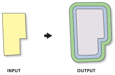
The Multi-Ring Buffer tool creates a series of dynamic, concentric buffer rings around point, line, or polygon features at multiple specified interval distances. Rather than running the standard buffer tool repeatedly and manually merging output datasets, the multi-ring buffer tool automates the generation of multiple distance bands in a single geoprocessing step.

Step-by-Step Execution: How to Use Multi Ring Buffer Tool in ArcGIS

Understanding how to use multi ring buffer tool in arcgis involves a clear sequence of configurations:

1. In ArcGIS Pro, open the Geoprocessing pane and search for “Multiple Ring Buffer”.
2. Set your Input Features layer (such as a city center or hazardous waste facility).
3. Define the Output Feature Class name and storage location.
4. In the Distances table parameter, enter each target distance offset sequentially (for example, 100, 250, 500, 1000).
5. Choose the Buffer Unit corresponding to your numerical inputs (such as Meters or Miles).
6. Select the Field Name where distance values will be recorded in the output attribute table (default is usually distance).
7. Choose the Dissolve Option:

• Overlapping (Don’t Dissolve): Retains complete concentric disks stacked atop one another.
• Non-overlapping (Rings): Converts the buffer rings into non-overlapping donut shapes, where each ring represents only the specific spatial band between two consecutive distance thresholds.

1. Click Run to generate your multi-band proximity model.

Multi-ring buffers are extensively used in accessibility modeling, noise pollution impact assessments around airports, wildfire evacuation risk bands, and retail catchment analyses.

Real-World Applications of Buffer Analysis in ArcGIS

The real-world practical applications of the ArcGIS buffer tool span across virtually every industry utilizing geospatial data and spatial analysis.

1. Environmental Protection and Riparian Management

Environmental regulators routinely use buffer analysis in ArcGIS to protect sensitive ecosystems. For instance, forestry management guidelines often mandate 100-foot protective riparian buffer zones along stream banks and wetlands to filter agricultural runoff, prevent soil erosion, and maintain aquatic habitats. By running a buffer on stream centerline vectors, environmental managers can overlay agricultural zoning layers to identify non-compliant land use zones.

2. Urban Planning and Public Transit Accessibility

Urban planners rely on fixed distance and multi-ring buffers to assess transit-oriented development (TOD). By generating 400-meter and 800-meter (roughly 5-minute and 10-minute walk times) buffer rings around subway stations or bus stops, planners can calculate pedestrian catchment areas, assess housing density within walk zones, and identify underserved neighborhoods lacking adequate public transit access.

3. Public Safety and Emergency Response Planning

During industrial hazardous material spills or chemical plant emergencies, emergency management agencies utilize geodesic buffering to establish immediate danger zones and secondary evacuation corridors. By buffering the incident point at prescribed safety radii, emergency responders can rapidly perform spatial intersections with land parcel layers to generate emergency notification call lists and evacuation route maps.

4. Commercial Real Estate and Retail Site Selection

Retail chain operators use variable distance and multi-ring buffers to analyze demographic profiles around potential new store locations. By creating 1-mile, 3-mile, and 5-mile buffer rings around site candidates, analysts extract total population, median household income, and consumer spending data within each ring to forecast revenue potential and avoid cannibalization of existing franchise stores.

Common Pitfalls and Troubleshooting Tips

While the ArcGIS buffer tool is straightforward to configure, spatial analysts frequently encounter common errors and performance bottlenecks. Here are key troubleshooting strategies to ensure optimal results:

1. Spatial Reference Mismatches and Distortion

• Problem: Buffer output polygons appear distorted, oval-shaped, or display incorrect distance measurements on the map display.
• Solution: Check the spatial reference of both your input feature layer and your active map frame. If your feature layer uses an unsuitable geographic coordinate system, standard planar buffering can introduce severe distortion. Reproject your dataset into a local Projected Coordinate System (PCS) prior to running planar buffers, or explicitly set the Buffer Method to Geodesic.

2. Unexpected Overlaps and Spatial Double-Counting

• Problem: Running downstream overlay operations (such as Summarize Within or Intersect) on multi-feature buffers produces inflated summary values due to overlapping geometries.
• Solution: Ensure you select the appropriate Dissolve Type during execution. Use “Dissolve All” or “Dissolve by Field” if your goal is to assess total geographic area without double-counting spatial intersections.

3. Performance Bottlenecks with Large Feature Layers

• Problem: Running buffer operations on extremely large vector datasets (such as millions of parcel boundaries or detailed stream networks) causes the tool to stall or run out of memory.
• Solution: Pre-filter or slice your input data into regional subsets prior to processing. If using “Dissolve All”, consider running the buffer tool with “No Dissolve” first, and then applying a separate Dissolve geoprocessing tool afterwards, as handling dissolvings in separate stages can optimize RAM consumption. Additionally, simplifying complex vector geometries before buffering can dramatically reduce computation times.

Conclusion

The ArcGIS buffer tool remains a fundamental pillar of modern GIS analysis and spatial modeling. From basic point proximity rings to complex, multi-band geodesic corridors, mastering this versatile geoprocessing tool enables spatial analysts to convert raw geographic features into actionable spatial intelligence.

By understanding the critical mathematical distinctions between planar and geodesic distance models, leveraging advanced parameters like end cap styles and dissolve options, and applying tools like the multi-ring buffer, you can execute rigorous, precise, and visually compelling proximity analysis in ArcGIS Pro. Whether you are conducting urban land-use evaluations, managing critical environmental resources, or optimizing logistics networks, applying proper buffering techniques ensures that your GIS workflows yield trustworthy and accurate analytical outcomes.